Quantum computing benchmarking
Core benchmark principles
Full system stack evaluation
Reproducible and transparent
Measuring time and quality
How performance is scored
TTS benchmarks measure the total wall time from job submission to a verified, qualifying answer. This covers the full pipeline from compilation through post-processing. Both types require a great underlying system. The difference is whether we measure time or quality as the output.
Results are reported per workload. A single aggregated benchmarking score cannot represent performance across problems that differ in structure, depth, and required accuracy.

Solution Quality

Time-to-Solution
Real-world results:
IonQ vs peers
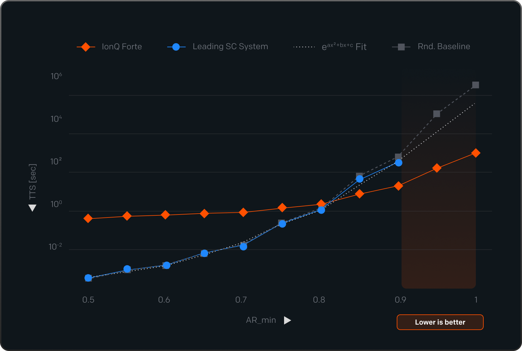
LR-QAOA
Linear-Ramp QAOA
IonQ’s system returns qualifying answers in seconds, even at the highest quality threshold (orange area). At that same quality bar, competing superconducting systems produce results statistically indistinguishable from random sampling, meaning the answers they return carry no useful signal and their Time-to-Solution can be considered “infinite”.
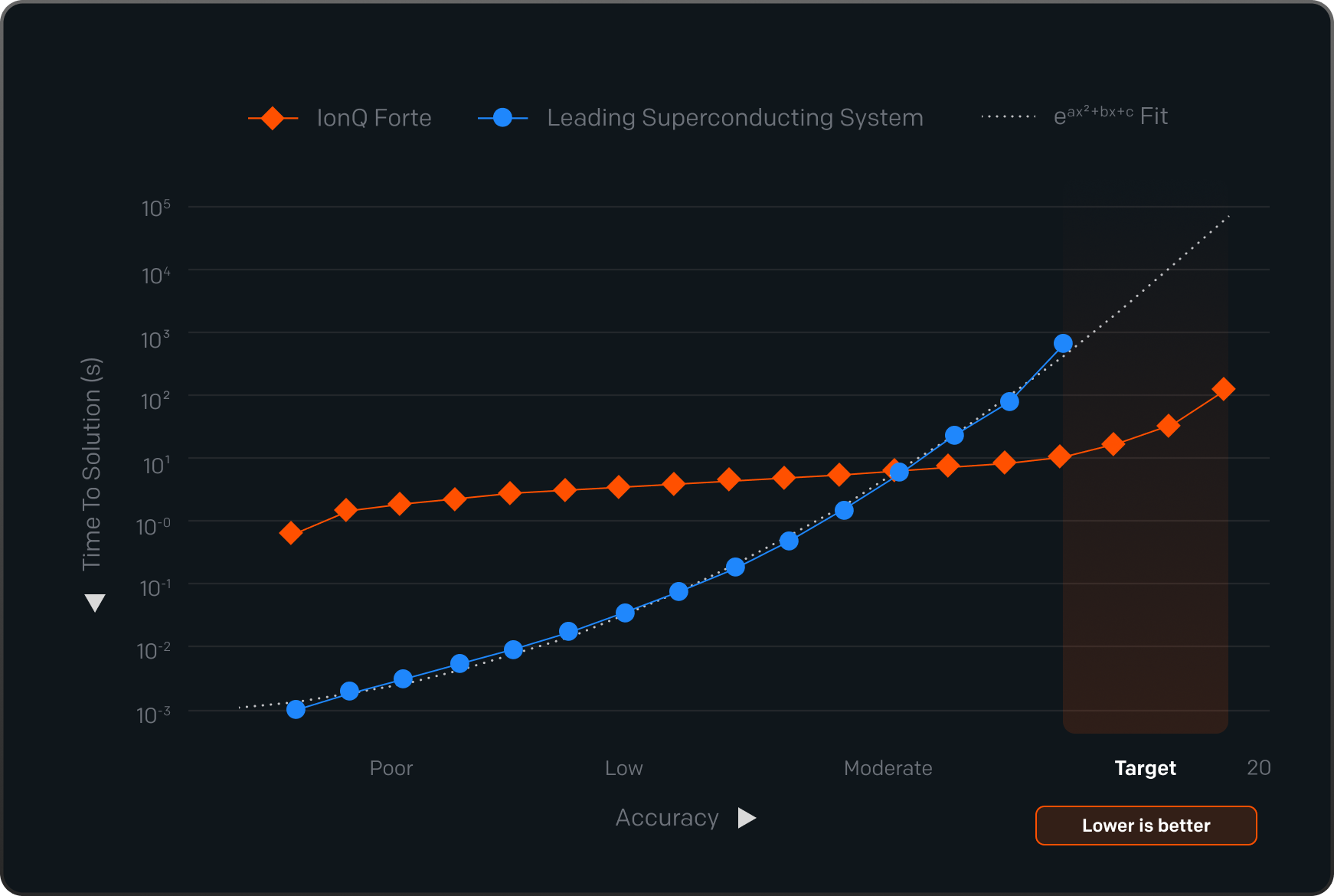
QFT Suite
Quantum Fourier Transform Suite
IonQ’s system maintains accuracy close to the ideal result across all tested circuit sizes. Competing systems degrade faster as circuits grow. At the largest sizes (orange area), the competing system’s scores approach what you would expect from a system dominated by noise, and Time-to-Solution becomes impossibly high.
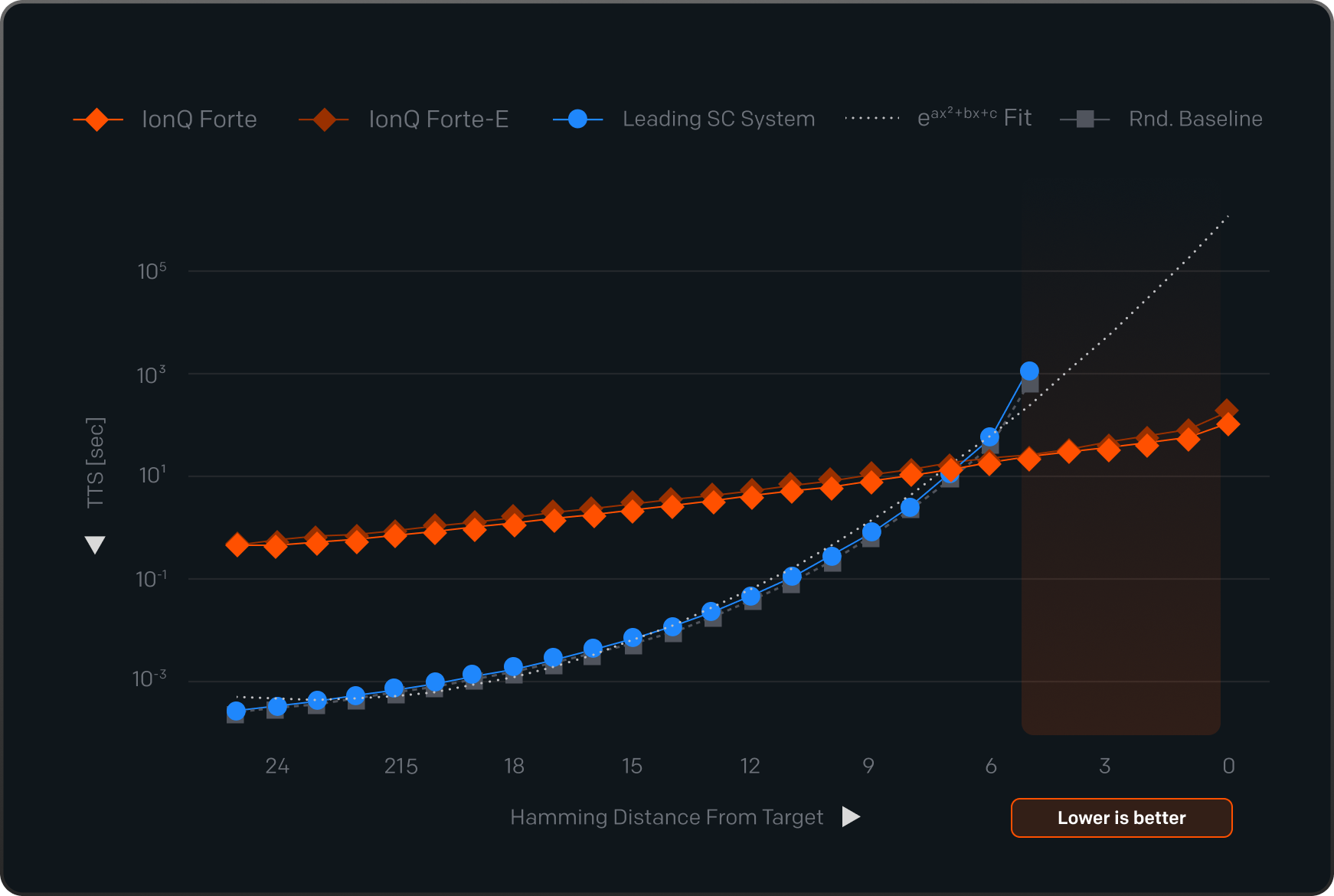
HSBP
Hidden Shift Benchmark Problem
IonQ’s systems return qualifying answers across the full range of quality requirements, including the hardest targets (orange area). Competing systems fail to produce valid results before reaching the highest bar, meaning they cannot complete this benchmark at the required standard for this problem size.
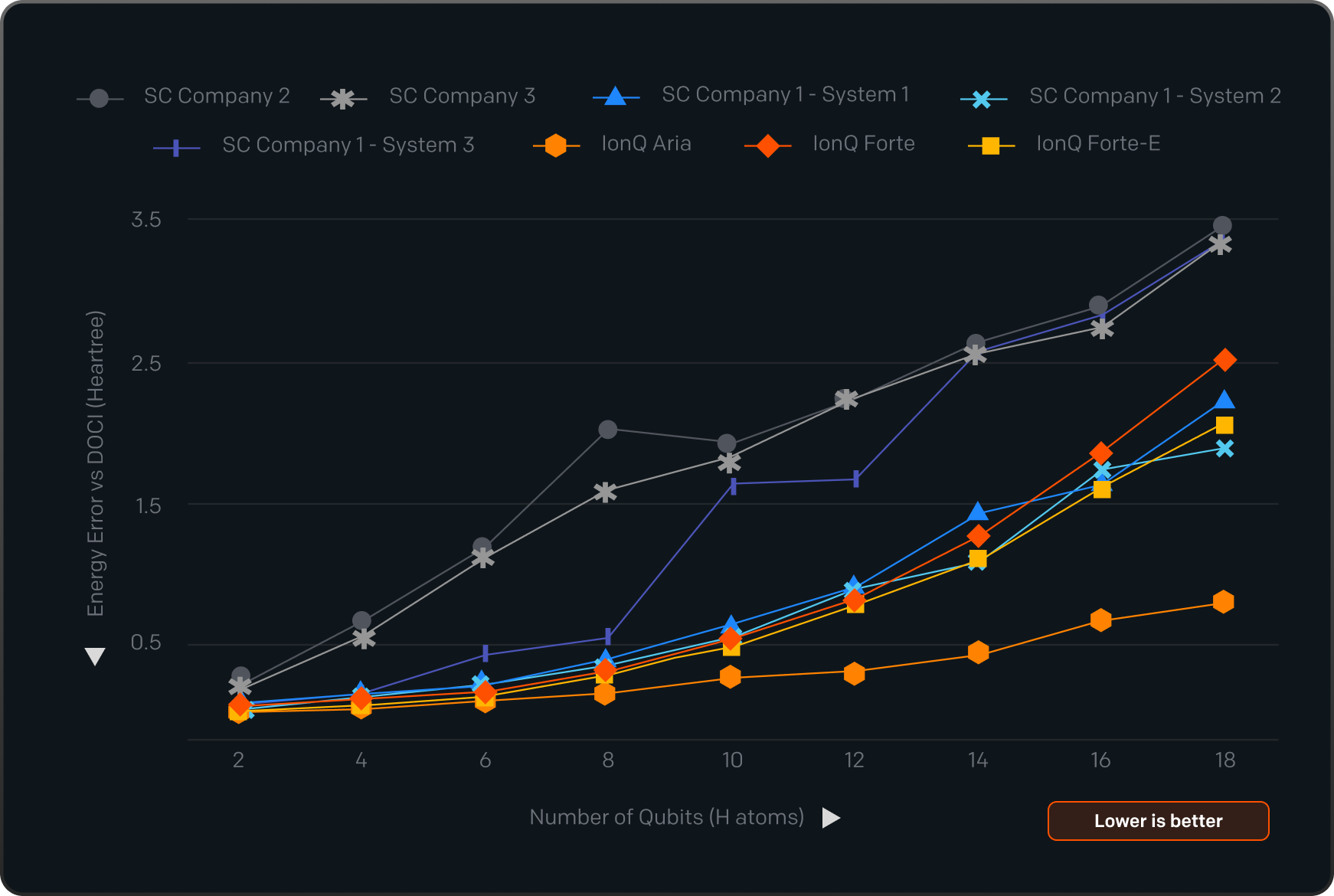
VQE
Variational Quantum Eigensolver
This benchmark scores solution quality rather than speed. The chart shows how far each system's answer drifts from the correct molecular energy as the problem grows. IonQ stays closest to that target across all molecule sizes. Competing systems diverge more steeply as complexity increases.
The quantum benchmark suite
Each benchmark’s code, which is designed to be fixed (the “closed” category), is publicly available for independent verification, while benchmarks in the “open” category are open for innovation, and other companies can come up with novel ways to address the benchmark challenge in the best way possible.
.svg.png)