Last November, Sonika Johri, IonQ’s Lead Quantum Applications Research Scientist, and Elton Zhu, Director of Quantum Research for the Fidelity Center for Applied Technology, gave a presentation at the NVIDIA GTC summit on their collaboration in quantum machine learning to simulate market behavior for financial applications. While this talk focuses on finance, the underlying generative techniques may be applicable in a variety of business contexts.
For those who want to dive deep into the details of this research, we present a condensed and clarified transcript of Sonika and Elton's presentation, which can also be watched in full here. The paper this talk is based on, Generative Quantum Learning of Joint Probability Distribution Functions, can be found here.
SONIKA: We are excited to present you the results of our research in the emerging field of quantum machine learning.
In brief, we developed quantum algorithms that can learn to produce samples from joint probability distributions, which is an important task in a wide variety of fields. In this paper, we present theoretical arguments for exponential advantage in our model's expressivities over classical models. We also show that the algorithms we developed outperform the equivalent classical generative learning algorithms on a variety of metrics when trained on IonQ quantum computers.
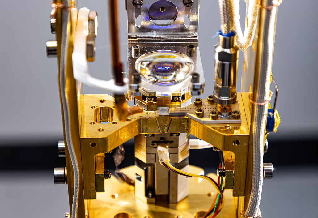
Let's begin with a brief introduction to trapped ion quantum computers. In general, quantum computers are based on quantum bits, or qubits, which can be in a superposition of zero and one at the same time. IonQ's qubits consist of ionized atoms, which are held in place by an electromagnetic potential, created using lasers.
.png)
During the computation, their state is manipulated by a series of operations called gates, which are implemented using laser beams. As the computation progresses, the quantum gates acting on certain qubits are physically realized by laser beams acting on the target ions. At the end, the qubits are let out with the help of the laser beam into a classical zero or one state.
Here is a photograph of the real trapped ions in one of IonQ's quantum computers. As you can see, they are arrayed in a linear fashion.
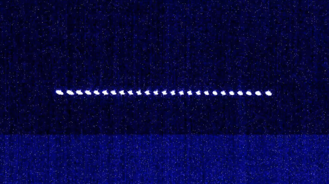
Note that one of the powerful features of our system is that despite the qubits being linearly arranged, gates between any two pairs of qubits in the array can be directly implemented with high fidelity. This correspondingly makes it a really attractive platform for running quantum algorithms with high accuracy. There are several additional benefits that are inherent to using ionized atoms as the basis for a quantum computer.
An important one is that atoms are fundamentally quantum, and each atom is given, by nature, to be the same as every other atom. Therefore they do not need difficult fabrication techniques with almost insurmountably high barriers to achieving high levels of uniformity and precision, which is really required for scaling the technology. The ions are isolated in space. They're far away enough from the substrate so that they're free of the influence of any defects in the substrate, as opposed to other solid-state qubits. The trapped ion chips do not require any special fabrication techniques or materials and can thus be manufactured in a commercial silicon fab, which, in turn, makes them relatively economical to manufacture.
Along with the benefits, based on the fundamental physics, IonQs systems also come with several architectural benefits. As I mentioned before, the systems have all-to-all connectivity, and gates can be run between any two pairs of qubits. The systems are completely optimized and continuously calibrated by us.
The user does not have to know anything about the physics of ions to program our quantum computers. This level of abstraction makes it really easy to get started with programming and developing applications on IonQ systems.
Elton Zhu, Director of Quantum Research, collaborated with Sonika and IonQ to develop an application demonstrating how our quantum hardware can be used to improve the analysis and prediction of stock performance.
ELTON: Let’s start by going through some of the high-level ideas of our joint paper with IonQ on generative quantum learning.
What is machine learning? Typically, we think of machine learning as some supervised task. You give a machine some data, and you ask it to figure out. For example, if you have a bunch of images between cats and dogs, but you don't have labels of them, and maybe what you want to do is try to label them into their corresponding species, or if you have some historical stock prices, and you may want to use that to predict the future stock price. However, that's not all of machine learning. The models that we refer to are called discriminative models.
There are mainly two kinds of discriminative models, classification and regression.
Classification, for example, helps identify spam in your inbox, can detect anomalies in a dataset, or could identify which images in a dataset are cats versus dogs. Regression looks at trends—it might predict stock prices, predict population growth, etc. However, there's another class of machine learning models called generative models that are getting increasingly popular. These generative models try to learn from the pattern in data and then try to generate synthetic data with the same pattern.
For example, it can be used to generate images, speech, text, and other kinds of data. You may have heard of a “deepfake,” and that is an example of an application of a generative model. Some of the most famous examples of generative models include Generative Adversarial Network, GAN, or VAE, Variational Autoencoder.
We think quantum computers are particularly suitable for generative models for several reasons.
Firstly, generating data is a much harder task than labeling data. As you can imagine, it's quite easy to differentiate between cats and dogs and put labels on them, but it's much harder to generate images of cats and dogs.
I'm talking about a situation where you generate the images yourself, not taking a photograph of a real cat or dog. Also, classical machine learning models have been exceptionally good at discriminative models. For example, facial recognition, or spam detection. Our classical machine-learning models have been doing that really well.
Near-term quantum computers, on the other hand, still have very significant noise, and some of them may have gate error up to four percent.
This means that if you ask a quantum computer to implement a logic gate, it could have as much as a 1 in 25 chance of failing at that. As a result, it is quite hard to imagine near-term, noisy quantum computers outperforming classical computers in discriminative models.
Generative models, however, represent a much more suitable task for quantum machine learning. This is because in discriminative models we're asking a model to generate a single output, a yes or no, in the case of classification. And also to generate a variable, a continuous variable, in the case of regression. But in generative models, we are asking the machine to generate a lot of data. For example, an image, like a one thousand pixel image, has many data.
A gate failure from a quantum computer may be analogous to a bad pixel in an image. The image has so many pixels that a bad pixel is probably okay, as long as the pattern, the overall pattern, is correct. The reason why a financial firm, like us, is interested in generative models because this can be used to improve backtesting of other financial models.
For example, we may want to build a machine-learning model that predicts the next day's stock price, based on its last thirty days of history. This is a completely sensible thing to do in a financial firm and we have five years of historical data available, from 2016 to 2021.
As usual, you divide your data into eighty percent training and twenty percent testing. At the start of the pandemic, which was March of 2019, that was a period of huge market volatility. If you have a trained model then a very natural question may be 'how does my model perform at the start of the pandemic?'
The thing is you probably can't know the answer because the data at the start of the pandemic falls under your training data. If it falls under your training data, then you can't use that for backtesting because that will create bias. So you may say, 'why can't I move that period into the testing so that I still create my model with the other training data, and I can backtest my model for this period?'
Sure. No problem. You can do that, but then your training data no longer include this period. Your model will not learn the market dynamics during this period of huge volatility. You can either use it for training or for backtesting but not both. This creates a dilemma.
One way of mitigating this issue is to use a generative model to generate synthetic financial data. Maybe some of them will mimic this kind of volatile market event. This will complement traditional backtesting. By doing that we can reduce the likelihood of our models overfitting and illuminate other potential model failures.
The thing is that you can use your generative models to simulate other types of volatile market events. There's also the financial crisis in 2008, and there are some other market events. If you have a lot of synthetic data then you can backtest your model in many ways, but there's one catch; the success of such a technique depends on the quality of the synthetic data.
If your data is trash then you can't get any value from your backtesting. Getting synthetic data of higher quality is always of interest. This brings us to the subject of GAN.
A GAN contains two neural networks, a generator and a discriminator. These two neural networks are trained alternatively in a zero-sum game.
Think of the generator as an art forger, who tries to forge 'previously unknown' paintings by great artists (not copies of existing works, but new fakes in the same style). Think of the discriminator as an art investigator, who tries to detect fake paintings. The art investigator will look at famous paintings which are known to be real, and then he will look at the paintings produced by this art forger, and then he will try to learn from that. The investigator will announce what paintings he has determined to be forged. Those announcements will provide useful feedback to the art forger.
After many, many iterations, the art forger will learn which of her paintings are good and which paintings are bad. Then she will probably be able to produce high-quality paintings. One thing to note is that during this process, the art forger never sees those original paintings by the great artists. The reason for that is because we're trying to let it learn how to paint -- not imitate.
It is easy to think that if the forger's work is as good as the real paintings, then she will pass the test and the investigator will never be able to tell that they are fakes. But that's not the point. We want the generator, the art forger, to generate new realistic famous paintings and not imitations.
Since the invention of GANs, there have been many interesting applications.
For example, one can take human images and try to generate the cartoon versions of them. You can take a picture of a model and then try to create other poses of the same person, who has the same clothes, or with different clothes. One can blend images together, like a polar bear in a desert, and with very smooth transitions.
.png)
Other applications include super-resolution of images and the text-to-image translation. In fact, Nvidia has done some of its own cutting-edge research in this space, with the famous StyleGan, which generates highly realistic human faces.
Making quantum GAN works means that the generator, our art forger, now becomes a quantum computer.
The model of the generator is no longer a neural network but some kind of a quantum circuit. The discriminator, or what we call the art investigator, is still a classical neural network. Of course, you could also use a quantum circuit to do that, but we're not trying to do that here. This is an example of a hybrid quantum/classical neural network because, in training, you have your quantum algorithm run for a period of time, and then you have the classical neural networks being trained. Then the classical neural networks will tell the quantum circuit how to improve, and then that will also train the classical discriminator.
It's this kind of quantum/classical feedback loop. This is an example of a quantum classical hybrid algorithm because it's not all quantum, it's not all classical. It's a hybrid algorithm.
Quantum GAN is not the only quantum generative model that one can build. There's another model which we call the Quantum Circuit Born Machine (QCBM).
This is a peculiar name. The objective of the model is still the same. It tries to generate very realistic paintings. However, the way that we train the model is slightly different. In this case, there is still the generator, but there's no more discriminator. What happens is that the generator will still generate paintings, but then there's a separate process which looks at this and compares that with the classical images.
It will try to minimize the similarity between them and tell that to the generator. As a dissimilarity measure, we typically use KL divergence, but you can use some other ones. In our paper, we defined these generative, quantum generative models for the purpose of learning and drawing the distributor data.
.png)
In this case, it's the daily return of Apple and Microsoft. We saw the hypothetical growth if you invest ten thousand dollars into either stock. Looking at the data over eight years' time, from 2010 to 2018. Over that period, the return of Apple is a little bit more volatile than that of Microsoft. Microsoft was pretty stable, but if you break down the data into the data return space then you'll see that it's a little bit noisy and it fluctuates around the zeroes, but sometimes there can be extreme events.
For example, having plus or minus five percent day-to-day return is a huge event that can usually occur. We use a technique in statistics called 'probability integral transform' to convert the data in the daily returns to the copula space. Once you do a conversion, the data is in the abstract space, but then there are some very nice features. For example, the range of your data is between zero to one, and it's always within zero to one, and also, the data is uniformly distributed in either axis.
Of course, if you look at the data in two axes together then you can still see some interesting patterns. The data of this form is very easy for a quantum computer to learn and we think that this kind of joint distribution corresponds to something in quantum computing called 'maximally entangled states.' So, we design our models with the following architecture: you have the classical GAN, which is our neural network, and then you have the discriminator for classical GAN and quantum GAN.
We do a control experiment. We use the same neural network architecture. Know that our generator, our classical GAN generator here is a very small neural network, and the reason is because we want to control the GAN and QGAN, the generator to be of the same level. So, we both allow twenty four parameters for the model.
.png)
Of course, you can use larger models, but that wouldn't be a fair comparison. Recall that in the quantum circuit machine, there's no more discriminator. There's no more learning rate for the discriminator, and then we have the epochs batch size learning rates. This is the quantum circuit that represents the quantum generator. Here, it starts from zero states, and then it applies the Hadamard gate and a bunch of CNOT gates, and then it applies the unitaries in both partitions.
This kind of a quantum circuit creates the maximally entangled states. Whenever you run a quantum circuit on a quantum computer, you make a measurement towards the end, and you can use those measurements to reconstruct a point of the daily return. That represents one day's daily return for either Apple or Microsoft's stock.
Let's say if I want to generate five hundred days of daily return, then you can run the same circuit five hundred times and make five hundred measurements. This will generate many different data points. The image shown below is a plot of the cost function for our QGAN training. The first one is from a simulator, and the second one is from IonQ's 11-qubit quantum computer, which, by the way, is commercially available.
.png)
The difference between the simulator and IonQ's quantum computer is that the simulator doesn't have any noise. If you ask it to do anything, it will do that perfectly, but IonQ's eleven qubit quantum computer still has a little bit of noise. If we look at the plot of the loss function, in both cases, we can see that the loss function of the generator is increasing in the beginning, while that of the discriminator is decreasing.
This can be interpreted as the discriminator getting better while the generator is lagging behind a little bit. The generator may still be improving, but it's just lagging behind the discriminator. This is not too surprising. You can think of it this way: it's relatively easy for the discriminator to learn how to distinguish between the real and the fake data, but it's much harder for the generator to actually generate data that is comparable to the training data.
You also see that, after a certain point, the two loss functions actually converge. This can be interpreted as some kind of an 'aha!' moment. When this 'aha!' moment occurs, the generator suddenly figures out the pattern of the data and learns very, very rapidly. After this convergence, the model training sort of enters a equilibrium phase, but we also see that the convergence from the experiment comes slightly later than as compared to a simulation.
This is because of the noise of the quantum computer. This noise makes it much harder for the quantum computer to learn. We also performed various statistical testing on the data that is being generated by all of these models. The statistical testing that we performed is called two-dimensional Kolmogorov‐Smirnov hypothesis testing, and we compared some classical models, the classical GAN model and another parametric model, and we have the quantum models both in simulation and experiments.
The lower the metric, the better it is. The metrics have a different range because one can use different initializations, and we observe that the smaller the model is, the better. You can see that in most cases the quantum models are better than the classical models, and also, we have the visualization of the data.
.png)
As you can see, the quantum models are a little bit more realistic. Also, one other interesting thing to note here is that in the classical GAN model, the model sort of only concludes after twenty thousand iterations, whereas in our quantum models the quantum GAN concluded after one thousand iterations, and the Quantum Circuit Born Machine only concludes in twenty eight iterations, which is really fast.
The reason why the Quantum Circuit Born Machine is able to converge much faster than a quantum GAN model is because, in a quantum GAN, you have this adversarial training between the generator and the discriminator. That typically takes more time, but in a lot of cases it's also more stable. We also argue, based on computational complexity theory, that the space of patterns that can be efficiently learned by a quantum computer is definitely more than the space of data that can be generated and efficiently learned classically.
.png)
The middle circle here represents all of the data patterns that can be efficiently learned using a quantum computer. You can use quantum GAN or a Quantum Circuit Born Machine, or you can invent your own quantum algorithms, but that middle circle represents the space of all data structures that can be learned that way. The smaller circle represents the space of patterns that can be modeled efficiently using a classical computer, and there's a separation between these two.
We show that there are structures which are easier for a quantum computer to learn, compared with a classical computer. Of course, you may ask, 'what if I want my classical computer to learn those data?' You can, but that is going to take exponential time. A quantum computer can learn from more complex structures within data, and it will take a classical computer exponential time to do that, and we call this 'exponential quantum advantage.'
We know that there are many other interesting features based on our research, for example, the probability of convergence. We trained our models, at least in simulation, using many different kinds of random initialization, and they almost always converge. However, for the classical GAN model that we built, again, we tried many different initializations, and in forty percent of the models, the models do converge.
In the other sixty percent of the cases, the model just collapsed and never learned from the data. Another interesting thing to note is the higher learning rate. In our quantum models, we can increase this learning rate to a very large magnitude, and this has the benefit of reducing the number of epochs in a training. This potentially makes your training much shorter.
We tried to do that for a classical GAN model, but whenever we increased the learning rate, the model becomes very volatile and it just doesn't learn very well.
We also did not observe any vanishing gradients. The vanishing gradient is a very common problem in classical GAN, but we did not observe that here. We demonstrated our generative model for two-dimensional data. We used it to model the data returns between Apple and Microsoft, but realistically you may have multidimensional data. Maybe you have ten columns or a hundred.
For our scheme, it's relatively easy to expand that to model such higher-dimensional data. Our circuit generates two-dimensional bipartite entangled states. You just have to generate multipartite entangled states, things like GHZ states. This will definitely require higher qubits, but otherwise there's no modification to the model.
We believe that our advantage still holds true on a large scale. If that's true, this could be an area of the first practical quantum advantage.