Getting started with Native Gates

The IonQ Quantum Cloud has one of the best—maybe the best—optimizing compilers in quantum computing. This allows users to focus on the details of their algorithms instead of the details of our quantum system. You can submit quantum circuits using a large, diverse set of quantum gates that allows for maximum flexibility in how to define your problem, and our compilation and optimization stack is designed to ensure that by the time it actually runs on hardware, it is a hardware-optimized and highly compact circuit, without ever having to worry about hardware or circuit optimization themselves.

This flexibility in circuit definition also allows for high portability of algorithm code. We don’t restrict you to hardware-native basis gates, so you’re free to define in any gate set you want—even the basis gates of a different hardware provider—and then simply submit to IonQ hardware as-is. No changes necessary!

While this is ideal for many applications-focused users, an abstract gate set is not ideal for certain researchers, academics, and other quantum experts trying to advance the field.

The hardware-native basis gate set allows for more customizability, flexibility, and what-you-submit-is-what-you-get control. Being as “close to the metal” as possible allows for control over each individual gate and qubit, unlocking avenues of exploration that are impossible with a compiler between you and the qubits.

We’re excited to share that we’ve now enabled this feature—previously only available to select research partners and customers—to anyone using the IonQ Quantum Cloud via an IonQ-provided API token, including those who access IonQ hardware through Google Cloud Marketplace. To allow users to build confidence and understanding in this new interface before they run jobs on QPUs, we’ve also expanded our quantum simulator service to enable simulations using the same native gate set. We are also working with other partners to enable this ability in more places in the coming months.

Read on to get started with our new hardware-native gate specification, learn how it works, and run an example circuit using this powerful new ability.

Contents

When To Use Native Gates
Introducing The Native Gates
Single-Qubit Gates
Entangling Gates
Using The Native Gates
Native Gate JSON Specification
Example Algorithm: Zero-Noise Extrapolation
Running On The Simulator
Running On The QPU
Converting to Native Gates
General Algorithm
Conversion in Code
Additional Resources
Contact Us

When To Use Native Gates

Native gates are not the right solution for every problem. As the warning above states, the native gate specification is an advanced-level feature. If your goal is simply to run a quantum circuit for evaluation or algorithm investigation purposes, using native gates will often result in lower-quality output than simply using the abstract gate interface.

The native gate interface is the simplest, most direct way to run a circuit on IonQ hardware: we run exactly the gates you submitted, as submitted, and we return the results. That’s it.

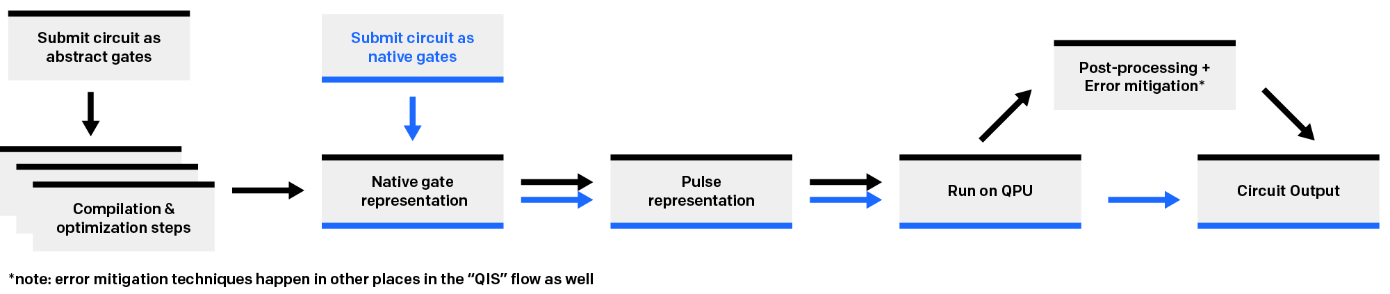
Comparison of submitting via the native gate interface (blue) and the abstract interface (black)

This means that our proprietary compilation and optimization toolchain and error mitigation tools are all off when we execute a “native” circuit. To take advantage of these tools, you must submit your circuit using our default abstract gate interface, and if you are looking for maximum algorithmic performance from our systems, it is likely that you’ll find it by doing just that.

But, this toolchain performs a number of transformations on submitted circuits that we consider proprietary, and we therefore do not disclose the full details of how it works. By the time a circuit you submit through the abstract gate interface actually runs on hardware, it has been changed, sometimes considerably. Extraneous gates are optimized away or commuted into different places, they are transpiled into native gates using special heuristics and optimized again, and so on.

So, we recommend only using native gates when you cannot use the abstract interface to accomplish your goals. Often, this means when you want to interact with the noise inherent in these NISQ devices in a very specific way that black-box optimization and error mitigation would interfere with, such as to make your circuits noise-aware, or to investigate the noise itself.

Perhaps you are working on your own compilation or error mitigation tools or contributing to open-source ones like those in Qiskit or Mitiq. Maybe you want to run back-to-back gates that would normally optimize away to explore zero-noise extrapolation, use a “no-op” gate as a check on the quality of a bell state, or train an ML model to produce noise-optimized circuits.

Maybe you just want to try your hand—or your students’ hands—at compiling and optimizing a circuit from its abstract representation to a native representation to see how it compares to our optimization and compilation stack.

These are the kinds of use cases where native gates shine.

Introducing the Native Gates

The native gate set is the set of quantum gates that are physically executed on IonQ hardware by addressing ions with resonant lasers via stimulated Raman transitions.

We currently expose two single-qubit gates and one two-qubit entangling gate. Other native gates may be provided in future.

Single-Qubit Gates

The “textbook” way to think about single-qubit gates is as rotations along different axes on the Bloch sphere, but another way to think about them is as rotations along a fixed axis while rotating the Bloch sphere itself.

Because, in physical reality, the Bloch sphere itself is rotating — that is, the phase is advancing in time — changing the orientation of the Bloch sphere is virtually noiseless on hardware. As such, the native interface is optimized for as much manipulation occurring in this “noiseless” phase space as possible.

GPi

The GPi gate can be considered a π or bit-flip rotation with an embedded phase. It always rotates π radians—hence the name—but can rotate on any longitudinal axis of the Bloch sphere. At a ϕ of 0 this is equivalent to an X gate, and at a ϕ of 0.25 turns (π/2 radians) it’s equivalent to a Y gate, but it can also be mapped to any other azimuthal angle.

$GPI (\phi)=\begin{bmatrix} 0 & e^{-i\phi}\\ e^{ i\phi} & 0 \end{bmatrix}$

It is physically implemented as a Rabi oscillation made with a two-photon Raman transition, i.e. driving the qubits on resonance using a pair of lasers in a Raman configuration. For more details on the physical gate implementation, we recommend this paper from the IonQ staff.

GPi2

The GPi2 gate could be considered an RX(π/2) — or RY(π/2) — with an embedded phase. It always rotates π/2 radians but can rotate on any longitudinal axis of the Bloch sphere. At a ϕ of π this is equivalent to RX(π/2), at a ϕ of 0.25 turns (π/2 radians) it’s equivalent to RY(π/2), but it can also be mapped to any other azimuthal angle.

$GPI2 (\phi)= \frac{1}{\sqrt{2}} \begin{bmatrix} 1 & -ie^{-i\phi}\\ -ie^{i\phi} & 1 \end{bmatrix}$

It is physically implemented as a Rabi oscillation made with a two-photon Raman transition, i.e. driving the qubits on resonance using a pair of lasers in a Raman configuration. For more details on the physical gate implementation, we recommend this paper from the IonQ staff.¹

Virtual Z

We do not expose or implement a “true” Z gate (sometimes also called a P or Phase Gate), where we wait for the phase to advance in time, but a Virtual RZ can be performed by simply advancing or retarding the phase of the following operation in the circuit. This does not physically change the internal state of the trapped ion at the time of its implementation; it changes the phases of the future operations such that it is equivalent to an actual Z-rotation around the Bloch sphere. In effect, virtual RZ operations are implied by the phase inputs to later gates.

$Virtual Z(\theta)= \begin{bmatrix} e^{-i\theta/2} & 0 \\ 0 & e^{i\theta/2} \end{bmatrix}$

For example, to add RZ(θ) — an RZ with an arbitrary rotation θ — to a qubit where the subsequent operation is GPI(0.5), we can just add that rotation to the phases of the following gates: --RZ(θ)--GPI(0.5)--GPI2(0) = --GPI(θ + 0.5)--GPI2(θ + 0). For a practical example, see the conversion code below.

Entangling Gates

For entangling gates, we offer two options: the Mølmer-Sørenson gate, and on our Forte-class systems, the ZZ gate.

Invented in 1999 by several groups simultaneously, the Mølmer-Sørenson gate along with single-qubit gates constitutes a universal gate set. By irradiating any two ions in the chain with a predesigned set of pulses, we can couple the ions’ internal states with the chain’s normal modes of motion to create entanglement.

For the Mølmer-Sørenson gate, we only offer two-qubit MS gates at this time. The fully entangling MS gate is an XX gate — a simultaneous, entangling, π/2 rotation on both qubits. Like our single-qubit gates, they nominally follow the X axis but take two phase parameters for additional flexibility.

While it is possible to entangle many qubits simultaneously with the Mølmer-Sørenson interaction via global MS, or GMS, we only offer two-qubit MS gates at this time.

Fully Entangling MS

The fully entangling MS gate is an XX gate — a simultaneous, entangling π/2 rotation on both qubits. Like our single qubit gates, they nominally follow the X axis as they occur, but take two phase parameters that make e.g. YY or XY also possible. The first phase parameter refers to the first qubit’s phase as it acts on the second one, the second refers to the second qubit’s phase as it acts on the first one.

If both are set to zero, there is no advancing phase between the two qubits because the transition is driven on both qubits simultaneously, in-phase. That is, the relative phase between the two qubits remains the same during the operation unless a phase offset is provided.

$\text{MS}(\phi_0, \phi_1)= \frac{1}{\sqrt{2}}\begin{bmatrix} 1 & 0 & 0 & -ie^{-i(\phi_0+\phi_1)} \\ 0 & 1 & -ie^{-i(\phi_0-\phi_1)} & 0 \\ 0 & -ie^{i(\phi_0-\phi_1)} & 1 & 0 \\ -ie^{i(\phi_0+\phi_1)} & 0 & 0 & 1 \end{bmatrix}$

Note that while two distinct phi parameters are provided here (one for each qubit, effectively), they always act on the unitary together. This means that there are multiple ways to get to the same relative phase relationship between the two qubits for this gate; two parameters just makes the recommended approach of “Virtual Z” phase accounting on each qubit across the entire circuit a little neater.

Partially Entangling MS

In addition to the fully entangling MS gate described above, we also support partially entangling MS gates, which are useful in some cases. To implement these gates, we add a third (optional) arbitrary angle θ:

$\text{MS}(\phi_0,\phi_1,\theta) = \begin{bmatrix} \cos \frac{\theta}{2} & 0 & 0 & -i e^{-i(\phi_0+\phi_1)} \sin \frac{\theta}{2} \\ 0 & \cos \frac{\theta}{2} & -i e^{-i(\phi_0-\phi_1)} \sin \frac{\theta}{2} & 0 \\ 0 & -i e^{i(\phi_0-\phi_1)} \sin \frac{\theta}{2} & \cos \frac{\theta}{2} & 0 \\ -i e^{i(\phi_0+\phi_1)} \sin \frac{\theta}{2} & 0 & 0 & \cos \frac{\theta}{2} \end{bmatrix}$

This parameter is also measured in turns, and can be any floating-point value between 0 (identity) and 0.25 (fully-entangling); in practice, the physical hardware is limited to around three decimal places of precision. Requesting an MS gate without this parameter will always run the fully entangling version.

ZZ Gate

The ZZ gate is another option for creating entanglement between two qubits. Unlike the Mølmer-Sørenson gate, the ZZ gate only requires a single parameter, θ, to set the phase of the entanglement. This makes it simpler to use in certain scenarios.

MS(ϕ₀,ϕ₁) and ZZ(θ) both provide the capability to entangle qubits, but they are implemented using different physical processes and offer different control parameters.

$ZZ(\theta) = \exp\left(-i \frac{\theta}{2} Z{\otimes}Z\right) = \begin{pmatrix} e^{-i \frac{\theta}{2}} & 0 & 0 & 0 \\ 0 & e^{i \frac{\theta}{2}} & 0 & 0 \\ 0 & 0 & e^{i \frac{\theta}{2}} & 0 \\ 0 & 0 & 0 & e^{-i \frac{\theta}{2}} \end{pmatrix}$

Due to the way our ion traps are physically designed, native ZZ gates are only possible on our Forte-class systems.

Why Use Arbitrary-Angle MS Gates?

More compact circuits
To produce the same effect as an arbitrary-angle MS would require as many as two fully-entangling MS gates plus four single-qubit rotations. This offers a potential reduction in gate depth that can indirectly improve performance by removing unnecessary gates in certain circuits.

Small-angle MS gates are generally more performant
Smaller-angle MS gates are realized by pulses with reduced power, and therefore experience lower light shift and other power-dependent errors. We do not currently have a detailed characterization of how much more performant these gates are on our current-generation systems, but in our (now-decommissioned) system described in this paper, we saw an improvement from ~97.5% to ~99.6% two qubit fidelity when comparing thetas of π/2 and π/100, which is described in more detail here.

Using the Native Gates

Native Gate JSON specification

This section provides a narrative explanation on the JSON native gate specification in the IonQ API. For instructions on using the native gate specification in a specific open-source SDK, see the guides on our IonQ Quantum Cloud Docs and Guides index, which include Using Native Gates with Cirq, Using Native Gates with Qiskit, and Using Native Gates with PennyLane.

If you have used our abstract gate specification, the native gate specification should feel quite familiar. Its parameters are slightly different though, and we’ll walk through them here.

Overview

To specify a circuit using native gates, you must do two things:

1. Set the parameter gateset to native inside the circuit body. This is an optional parameter that defaults to qis, which signifies our abstract gate set based on the general-purpose gates of quantum information science (QIS).

2. Your circuitarray must only use native gates, which take a slightly different set of parameters, described below.

gate

This is a string representation of the gate name — it works just like the abstract gate interface, but you can only use the three available native gates —gpi gpi2 and ms. If you submit any other gates in the array, you’ll receive an error.

phase

This is a number representation of the phase parameter or parameters in the gate. It is represented in turns, i.e. multiples of a full 2π rotation around Z.

So, π/2 radians = 0.25 turns, π radians = 0.5 turns, 3/2π radians = 0.75 turns, and so on. We accept floating point values between -1 and 1 for this parameter—anything larger than 1 turn can be simplified into fewer turns.

Why do we do this? We track the phase at the pulse level as units of turns — or, more accurately, as units of how long a turn takes — so, we expose the controls in the same way to you. This reduces floating point conversion error between what you submit and what runs.

The number index (starting from zero) of the qubit to apply the gate to. If the gate is a multi-target gate (i.e. the MS gate), use an array of qubit indices labeled targets instead.

A note on qubit topology and qubit routing: as a reminder, IonQ systems have all-to-all connectivity. Because of the highly dynamic nature of trapped-ion systems, we do not offer the ability to specifically select a single ion by its position in the chain. That is, qubit 0 is not guaranteed to be at any specific place in the ion chain — it may be on an end, in the middle, or at some other arbitrary place.

At the hardware control layer, the mapping from virtual to physical qubit changes from time to time based on certain parameters such as systematic drift, laser and optical characterization, and similar.

We do not guarantee a duration for which these mappings will remain consistent, or publish any updates when they change. That said, in practice, it’s fairly infrequent.

That is, we do not do any dynamic mapping at runtime on circuits submitted via our native gate interface. Within a single experiment or set of experiments run in a reasonably-narrow duration of time — think days, not hours — you can trust that a single qubit as-mapped will always be the same qubit.

Example Algorithm: Zero-Noise Extrapolation

As our example, we’ll implement a simple circuit that could be part of a larger Zero Noise Extrapolation (ZNE) experiment.

ZNE is an error mitigation approach that attempts to correct for noise in a gate or circuit by first creating a progressively noisier version of the circuit or subcircuit and then using this to extrapolate what the noiseless version would be. This is done by a technique called circuit folding — repeatedly running copies of the circuit and its inverse, to compound and observe the noise that this specific circuit creates. Both local folding (at the gate level) and global folding (at the circuit level) are possible.

For example, you might have a simple circuit to produce a bell state, which is just a single MS:

q_0 ----|         |----| M |
        | MS(0,0) |
q_1 ----|         |----| M |

In our JSON spec, this would look like:

zne-zero-folds.json

{
    "lang": "json",
    "shots": 100,
    "target": "simulator",
    "name": "zne ms - zero folds",
    "body": {
        "gateset": "native",
        "qubits": 2,
        "circuit": [
            {
                "gate": "ms",
                "targets": [0, 1],
                "phases": [0, 0]
            }
        ]
    }
}

To perform ZNE, you would add repetitions of this sequence and its inverse, canceling out the gate but leaving the observed noise. Abstractly, a unitary U

----| U |----

becomes

----| U |----| U† |---- ... ----| U |----

Adding additional pairs of U and U^† to scale the noise but maintain the same outcome until you have a full characterization, from which you can then extrapolate the point at which it has zero noise and apply this as an error mitigation technique.

For our circuit, MS with no phase is its own inverse, so we can add pairs of them to produce this effect:

----|         |----|         |----|         |----|         |----|         |----| M |
    | MS(0,0) |    | MS(0,0) |    | MS(0,0) |    | MS(0,0) |    | MS(0,0) |
----|         |----|         |----|         |----|         |----|         |----| M |

In our abstract gate interface, U U^† pairs like this are intelligently optimized away — because they collapse to identity, we don’t need to run them to produce the desired algorithmic outcome, and the fewer gates overall we run, the less we see the impact of gate noise.

This would ruin our ZNE experiment, where the repeated identities and their resulting noise are exactly what we want to identify and characterize.

In JSON:

zne-two-folds.json

{
    "lang": "json",
    "shots": 100,
    "target": "simulator",
    "name": "zne ms - two folds",
    "body": {
        "gateset": "native",
        "qubits": 2,
        "circuit": [
            {
                "gate": "ms",
                "targets": [0, 1],
                "phases": [0, 0]
            },
            {
                "gate": "ms",
                "targets": [0, 1],
                "phases": [0, 0]
            },
            {
                "gate": "ms",
                "targets": [0, 1],
                "phases": [0, 0]
            },
            {
                "gate": "ms",
                "targets": [0, 1],
                "phases": [0, 0]
            },
            {
                "gate": "ms",
                "targets": [0, 1],
                "phases": [0, 0]
            }
        ]
    }
}

Note that in a real ZNE experiment, you would repeat versions of this circuit for many iterations with different numbers of the U U^† pairs — this is just one example of that.

Running On The Simulator

If we save the above two snippets as named above — zne-zero-folds.json and zne-two-folds.json— running them on the simulator is as simple as submitting these two JSON job bodies to the API.

Putting the following two snippets in bash scripts called submit-job.sh and retrieve-job.sh will make your life a little easier when working directly from the command line.

submit-job.sh

curl -X POST "https://api.ionq.co/v0.2/jobs" \
-H "Authorization: apiKey $1" \
-H "Content-Type: application/json" \
-d @$2

retrieve-job.sh

curl "https://api.ionq.co/v0.2/jobs/$2" \
-H "Authorization: apiKey $1"

Now let’s run our jobs on the native gates simulator.

submit-job.sh YOUR_API_KEY_HERE zne-zero-folds.json

{
    "id":"7e932df8-6c7d-4fd9-a1de-f4ea19cccf3a",
    "status":"ready",
    "request":1652235779
}

submit-job.sh YOUR_API_KEY_HERE zne-two-folds.json

{
    "id":"91f8ca41-3307-4c4a-bd78-6a467dc71843",
    "status":"ready",
    "request":1652235801
}

Because the native gate simulator is an ideal simulator, the goal is to make sure that we wrote our circuits correctly and that they’ll execute correctly on the QPU — we won’t see any effects of compounding noise.

retrieve-job.sh YOUR_API_KEY_HERE f62999e1-b595-4388-84c6-78b2862c7186

{
    "status":"completed",
    "name":"zne ms - zero folds",
    "target":"simulator",
    "predicted_execution_time":4,
    "execution_time":0,
    "id":"7e932df8-6c7d-4fd9-a1de-f4ea19cccf3a",
    "qubits":2,
    "type":"circuit",
    "request":1652235779,
    "response":1652235781,
    "gate_counts":{"1q":0,"2q":1},
    "data":{
        "histogram":{"0":0.5,"3":0.5},
        "registers":null
    }
 }

retrieve-job.sh YOUR_API_KEY_HERE 91f8ca41-3307-4c4a-bd78-6a467dc71843

{
    "status":"completed",
    "name":"zne ms - two folds",
    "target":"simulator",
    "predicted_execution_time":4,
    "execution_time":0,
    "id":"91f8ca41-3307-4c4a-bd78-6a467dc71843",
    "qubits":2,
    "type":"circuit",
    "request":1652235801,
    "response":1652235802,
    "gate_counts":{"1q":0,"2q":5},
    "data": {
        "histogram":{"0":0.5,"3":0.5},
        "registers":null
    }
}

Looks like everything works and our jobs processed correctly — time to run on the QPU!

Running On The QPU

Running on a QPU via the native gate interface works the same as running on the simulator. We just need to change the target in our json job bodies to point at a QPU backend

{
    "lang": "json",
    "shots": 100,
    "target": "qpu.harmony",
    ...rest of job body
}

and submit them

submit-job.sh YOUR_API_KEY_HERE zne-zero-folds.json

{
    "id":"bf02bf25-f2ce-4d36-b2fd-1e20aeb5f9b3",
    "status":"ready",
    "request":1652237503
}

submit-job.sh YOUR_API_KEY_HERE zne-two-folds.json

{
    "id":"344da3d9-8cb9-4880-a5f0-4adf3163303e",
    "status":"ready",
    "request":1652237540
}

for comparison, let’s also run a version of our “two-folds” circuit through the abstract interface:

zne-two-folds-qis.json

{
    "lang": "json",
    "shots": 100,
    "name": "zne ms - two folds - abstract gateset",
    "target": "qpu.harmony",
    "body": {
        "gateset": "qis",
        "qubits": 2,
        "circuit": [
            {
                "gate": "xx",
                "targets": [0, 1]
            },
            {
                "gate": "xx",
                "targets": [0, 1]
            },
            {
                "gate": "xx",
                "targets": [0, 1]
            },
            {
                "gate": "xx",
                "targets": [0, 1]
            },
            {
                "gate": "xx",
                "targets": [0, 1]
            }
        ]
    }
}

submit-job.sh YOUR_API_KEY_HERE zne-two-folds-qis.json

{
    "id":"d8275b7b-62bf-4226-90be-735a5f514a37",
    "status":"ready",
    "request":1652237869
}

Now, let’s look at the results:

retrieve-job.sh YOUR_API_KEY_HERE bf02bf25-f2ce-4d36-b2fd-1e20aeb5f9b3

{
    "status": "completed",
    "name": "zne ms - zero folds",
    "target": "qpu.harmony",
    "shots": 100,
    "predicted_execution_time": 1929,
    "execution_time": 2464,
    "id": "bf02bf25-f2ce-4d36-b2fd-1e20aeb5f9b3",
    "qubits": 2,
    "type": "circuit",
    "request": 1652237503,
    "start": 1652237849,
    "response": 1652237851,
    "gate_counts": {
        "1q": 0,
        "2q": 1
    },
    "data": {
        "histogram": {
            "0": 0.45,
            "1": 0.02,
            "2": 0.01,
            "3": 0.52
        },
        "registers": null
    }
}

retrieve-job.sh YOUR_API_KEY_HERE 91f8ca41-3307-4c4a-bd78-6a467dc71843

{
    "status": "completed",
    "name": "zne ms - two folds",
    "target": "qpu.harmony",
    "shots": 100,
    "predicted_execution_time": 2199,
    "execution_time": 2517,
    "id": "344da3d9-8cb9-4880-a5f0-4adf3163303e",
    "qubits": 2,
    "type": "circuit",
    "request": 1652237540,
    "start": 1652237852,
    "response": 1652237854,
    "gate_counts": {
        "1q": 0,
        "2q": 5
    },
    "data": {
        "histogram": {
            "0": 0.34,
            "1": 0.1,
            "2": 0.12,
            "3": 0.44
        },
        "registers": null
    }
}

As we can see, the two-fold example has similar characteristics as the zero-fold example, but moreso. A slight weighting towards our |11> state becomes more apparent, and our total population in unintended states also goes up by about a factor of 10. If we were to continue adding folds, we would likely see these errors continue to grow in a similar fashion — we recommend you try it yourself and see!

Finally, let’s look at our two-fold circuit submitted via the “standard” abstract interface:

retrieve-job.sh YOUR_API_KEY_HERE 91f8ca41-3307-4c4a-bd78-6a467dc71843

{
    "status": "completed",
    "name": "zne ms - two folds - abstract gateset",
    "target": "qpu.harmony",
    "shots": 100,
    "predicted_execution_time": 2199,
    "execution_time": 2040,
    "id": "d8275b7b-62bf-4226-90be-735a5f514a37",
    "qubits": 2,
    "type": "circuit",
    "request": 1652237869,
    "start": 1652238466,
    "response": 1652238468,
    "gate_counts": {
        "2q": 5
    },
    "data": {
        "histogram": {
            "0": 0.48,
            "1": 0.02,
            "2": 0.01,
            "3": 0.49
        },
        "registers": null
    }
}

It looks more like our zero-folds example than our two-folds example, because after compilation, it was more like our zero-folds example — the folds were compiled away!

Converting to Native Gates

A new universal gate set that is subtly different from the “textbook” CNOT and X gates you might find in Nielsen and Chuang can be a little tough to begin wrapping your head around. To close this introduction to IonQ’s native gate set, we’ll discuss a few tools and techniques for taking circuits and making them work with our native gates.

General Algorithm

To translate anything into native gates, the following general approach works well:

1. Decompose the gates used in the circuit so that each gate involves at most two qubits.

2. Convert all easy-to-convert gates into RX, RY, RZ, and CNOT gates.

3. Convert CNOT gates into XX gates using the decomposition described here and at the bottom of this section.

4. For hard-to-convert gates, first calculate the matrix representation of the unitary, then use either KAK decomposition or the method introduced in this Phys, Rev. A. paper to implement the unitary using RX, RY, RZ and XX. Note that Cirq and Qiskit also have subroutines that can do this automatically, although potentially not optimally. See cirq.linag.kak_decomposition and qiskit.quantum_info.TwoQubitBasisDecomposer.

5. Write RX, RY, RZ and XX into GPi, GPi2 and MS gates as documented above.

Broadly speaking, this will produce a circuit where further optimization for total gate count is possible (and encouraged!), but it will be functionally equivalent to the circuit you start with.

CNOT to XX decomposition

----x-----   ----| RY(π/2) |----|         |----| RX(-π/2) |----| RY(-π/2) |-----
    |      =                    | XX(π/4) |                      
----@-----   -------------------|         |----| RX(-π/2) |---------------------

Many more advanced approaches, decompositions, and optimizations for trapped-ion native gates, including a parameterizable version of this decomposition can be found in Basic circuit compilation techniques for an ion-trap quantum machine, where this decomposition is described.

Conversion in Code

Writing RX, RY, RZ, and XX gates into native gates can still be a challenge. Here we provide an example code snippet that automatically converts a Cirq circuit made of these four gates into their native equivalents. The key here is to use a qubit_phase list to track and adjust the orientation of the Bloch sphere of each qubit as the circuit progresses. See this guide for more details on using native gates with Cirq.

from cirq_ionq.ionq_native_gates import GPIGate, GPI2Gate, MSGate
import numpy as np

def compile_to_native_json(circuit):
    qubit_phase=[0]*32
    op_list=[]
    for op in circuit.all_operations():
        if type(op.gate)==cirq.ops.common_gates.Rz:
            qubit_phase[op.qubits[0].x]=(qubit_phase[op.qubits[0].x]-op.gate._rads/(2*np.pi))%1

        elif type(op.gate)==cirq.ops.common_gates.Ry:
            if abs(op.gate._rads-0.5*np.pi)<1e-6:
                op_list.append(
                    GPI2Gate(phi=(qubit_phase[op.qubits[0].x]+0.25)%1).on(op.qubits[0].x)
                )
            elif abs(op.gate._rads+0.5*np.pi)<1e-6:
                op_list.append(
                    GPI2Gate(phi=(qubit_phase[op.qubits[0].x]+0.75)%1).on(op.qubits[0].x)
                    )
            elif abs(op.gate._rads-np.pi)<1e-6:
                op_list.append(
                    GPIGate(phi=(qubit_phase[op.qubits[0].x]+0.25)%1).on(op.qubits[0].x)
                )
            elif abs(op.gate._rads+np.pi)<1e-6:
                op_list.append(
                    GPIGate(phi=(qubit_phase[op.qubits[0].x]+0.75)%1).on(op.qubits[0].x)
                )
            else:
                op_list.append(
                    GPI2Gate(phi=(qubit_phase[op.qubits[0].x]+0)%1).on(op.qubits[0].x)
                )
                qubit_phase[op.qubits[0].x]=(qubit_phase[op.qubits[0].x]-op.gate._rads/(2*np.pi))%1
                op_list.append(
                    GPI2Gate(phi=(qubit_phase[op.qubits[0].x]+0.5)%1).on(op.qubits[0].x)
                )

        elif type(op.gate)==cirq.ops.common_gates.Rx:
            if abs(op.gate._rads-0.5*np.pi)<1e-6:
                op_list.append(
                    GPI2Gate(phi=(qubit_phase[op.qubits[0].x]+0)%1).on(op.qubits[0].x)
                )
            elif abs(op.gate._rads+0.5*np.pi)<1e-6:
                op_list.append(
                    GPI2Gate(phi=(qubit_phase[op.qubits[0].x]+0.5)%1).on(op.qubits[0].x)
                )
            elif abs(op.gate._rads-np.pi)<1e-6:
                    op_list.append(
                    GPIGate(phi=(qubit_phase[op.qubits[0].x]+0)%1).on(op.qubits[0].x)
                )
            elif abs(op.gate._rads+np.pi)<1e-6:
                op_list.append(
                    GPIGate(phi=(qubit_phase[op.qubits[0].x]+0.5)%1).on(op.qubits[0].x)
                )
            else:
                op_list.append(
                    GPI2Gate(phi=(qubit_phase[op.qubits[0].x]+0.75)%1).on(op.qubits[0].x)
                )
                qubit_phase[op.qubits[0].x]=(qubit_phase[op.qubits[0].x]-op.gate._rads/(2*np.pi))%1
                op_list.append(
                    GPI2Gate(phi=(qubit_phase[op.qubits[0].x]+0.25)%1).on(op.qubits[0].x)
                )
        
        elif type(op.gate)==cirq.ops.parity_gates.XXPowGate:
            if op.gate.exponent>0:
                op_list.append(
                    MSGate(
                        phi_0=qubit_phase[op.qubits[0].x], 
                        phi_1=qubit_phase[op.qubits[1].x]
                    ).on(op.qubits[0].x,op.qubits[1].x)
                )
            else:
                op_list.append(
                    MSGate(
                        phi_0=qubit_phase[op.qubits[0].x], 
                        phi_1=(qubit_phase[op.qubits[1].x]+0.5)%1
                    ).on(op.qubits[0].x,op.qubits[1].x)
                )
    return op_list

Additional Resources

Best Practices for Using IonQ Hardware has additional explanations and recommendations highly relevant to native gate users.

This introduction used our raw API, but in practice we recommend using a popular open source SDK for circuit synthesis and submission to our hardware. There are quickstart guides for the three that currently support native gates: Using Native Gates With Cirq, Using Native Gates With PennyLane and Using Native Gates With Qiskit.

For those interested in learning more about trapped-ion quantum computers as a physical apparatus, the implementation of gates, etc, we recommend the PhD theses from our cofounder Chris Monroe’s lab as a starting point, especially those of Debnath, Egan, Figgat, Landsman, and Wright. The hardware they describe is in many ways the “first iteration” of IonQ’s hardware, and much of the fundamental physics of the trapped-ion approach carries over.

Contact Us

Having trouble? Seeing something you don’t expect? Have other questions? Reach out to [email protected].

1 Note that this paper specifically describes IonQ Harmony, our 11-qubit system. In IonQ Aria, the Raman architecture replaces the global beam for two fans of individually addressing beams. This helps reduce certain sources of noise, but has the same physical effect on the ions.↫

Share on social media

Copied To Clipboard